Center of Mass Imaging

Note

Demonstration with the MoS2 dataset from the 4D-Explorer test dataset

Center of Mass Imaging (CoM) is a method used to reconstruct sample images from 4D-STEM datasets. The scientific principle behind CoM imaging is based on the deflection effect of the sample’s electric field on the electron beam. When the electron beam passes through the sample, the electric field causes deflections, and these deflections can be quantified by calculating the center of mass (CoM) of the diffraction patterns. The CoM reflects the projected electric field distribution of the sample. Specifically, CoM imaging calculates the center of mass for each scan position’s diffraction pattern and maps these CoM positions back into the sample space, resulting in a 2D image. CoM imaging is highly sensitive to weak scattering signals. Additionally, iCoM (Integrated CoM) and dCoM (Differential CoM) can also be computed, corresponding to the sample’s potential and charge density, respectively. iCoM is calculated by integrating the CoM of the diffraction patterns, while dCoM is obtained by differentiating the CoM to reveal the sample’s charge density distribution.

To reconstruct the 4D-STEM dataset, locate the dataset in the left panel, right-click on it, and select Reconstruction -> Center of Mass Imaging from the menu. In the Domain Shape dropdown at the top right corner, you can select the shape of the region to be included in the CoM calculation, such as circular or annular regions. After selecting the region type, you can adjust the parameters below, such as the radius and center coordinates. For CoM imaging, the circular region should at least cover the bright-field diffraction disk, or you can set the region radius large enough to cover the entire diffraction pattern.

If you are not satisfied with the appearance of the region (e.g., color or transparency), click the Adjust Effects... button. In the dialog that opens, you can modify the transparency (Alpha), edge color (Edge Color), interior color (Face Color), fill pattern (Hatch), line style (Line Style), and line width (Line Width), and choose whether to fill the region.

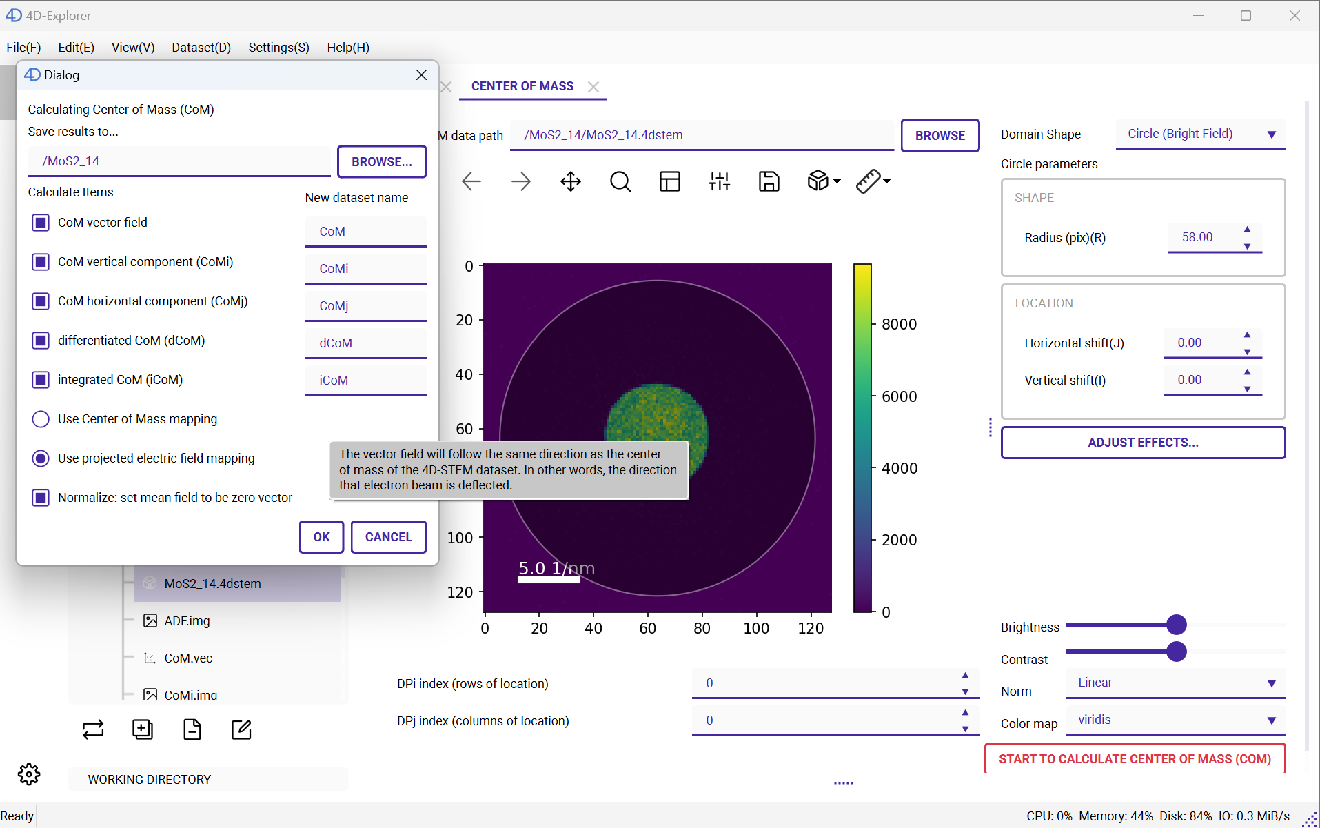
After selecting the integration region, click the red Start Calculation button at the bottom of the page. Choose the output image path and enter the names for the various images you wish to generate. Note that multiple image types can be generated at once, including the CoM vector field, its two components (as 2D images), iCoM, and dCoM. Each image type has a field next to it where you can specify the name of the output image. At the top of the dialog, you can specify the Group where these images will be saved. You can also select whether to use Center of Mass mapping or Projected electric field mapping. The latter corresponds to the electric field direction from high potential to low potential, consistent with the expected electric field strength. Additionally, you can check the Normalization box to set the average field strength to zero, preventing the appearance of a uniform, directional background field that might affect iCoM imaging. Once all settings are configured, click OK to begin the calculation.